ReplicantGuard: Building Age-Appropriate Content Safety Part 2
In Part 1 I walked through the text pipeline with how ReplicantGuard uses lexical scanning, TF-IDF contextual classification, and readability analysis to score written content against age-band profiles. This is done using no external models, is fully deterministic and is completely explainable.
flowchart TD
    subgraph Row1[ ]
        direction LR
        DASH[Dashboard]
        APPS[Apps]
    end

    DASH --> GATEWAY["⠀⠀⠀⠀⠀⠀Gateway⠀⠀⠀⠀⠀⠀"]
    APPS --> GATEWAY

    subgraph Services[ ]
        direction LR
        A[ODE Auth]
        B[ReplicantCore]
        C[ReplicantResonance]
        D[ReplicantGuard]
        E[ReplicantNarrative]
    end

    GATEWAY --> A
    GATEWAY --> B
    GATEWAY --> C
    GATEWAY --> D
    GATEWAY --> E

    %% --- Highlighting Styles ---
    classDef highlight fill:#ffd966,stroke:#b8860b,stroke-width:2px,color:#000;
    classDef faded fill:#e0e0e0,stroke:#999,color:#666;

    %% --- Apply classes ---
    class D highlight;
    %% --- class DASH,APPS,GATEWAY,A,C,D faded;
The same philosophy carries through to the other two pipelines and this post covers how ReplicantGuard scores images - what signals it looks for, how it extracts them, and why those signals map to specific content categories. In the next post which will be out soon, We will look at audio which completes the three pipelines ReplicantGuard currently supports.
The image pipeline
Much like text, Images pass through five layers before producing a category score, and each layer builds on the last.
I’ve taken a dependency on Pillow which is used to handle the image decoding only. Everything else - the colour maths, the edge operator, the flood-fill, the shape detection - is implemented from scratch.
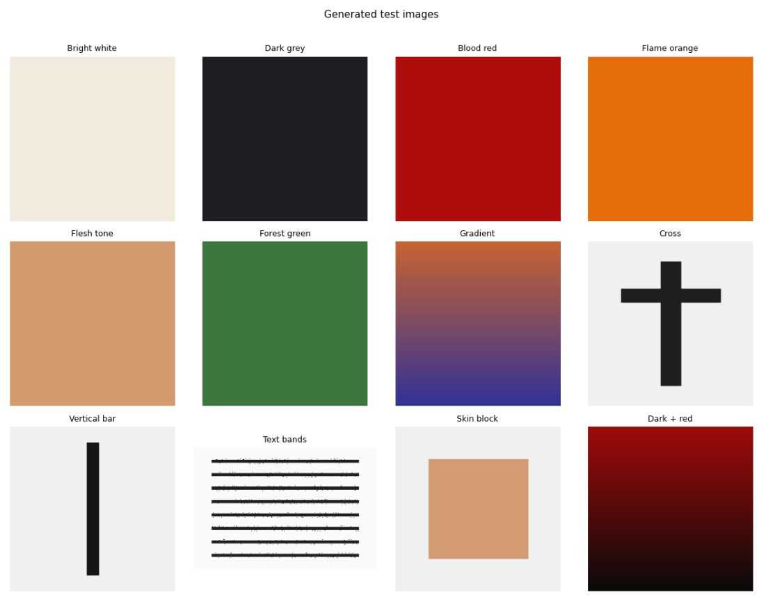
For the jupyter notebook examples, I have written code that generates test images that we will feed into the pipeline, and these look like this
Sampling strategy
Processing every pixel of every image would be expensive. if an image is in HD format (1920 x 1080) that would be 2,073,600 pixels to process.
The pipeline uses two sampling resolutions:
- COLOUR_STEP (4) - samples every 4th pixel in both axes, giving 1/16th of the image. Used for colour classification, edge analysis, and shape detection.
- BLOB_STEP (8) - a coarser 1/64th grid. Used for the flood-fill in Layer 3, where BFS traversal costs matter.
For a 1024×1024 image, that’s ~129,600 pixels at the fine resolution and ~32,400 at the coarse. Fast enough to run synchronously on the server, accurate enough to catch what matters.
Layer 1 - Colour
Every sampled pixel is converted from RGB to HSV. HSV is a much better colour space for this kind of classification than RGB - you can describe “skin tone” as a hue and saturation range without worrying about how bright the image is.
The conversion is the standard formula: hue in degrees (0–360°), saturation and value both 0–1.
Three colour classes are detected:
Skin tone covers the full Fitzpatrick scale from pale to darker complexions:
H ≤ 50° or H ≥ 330°   (warm reds and oranges wrapping around)
S between 0.08 and 0.72  (not too grey, not too saturated)
V between 0.20 and 1.0   (not too dark)
The wide hue range is intentional - it captures the orange-pink of lighter skin and the red-brown of darker skin in the same band. The saturation floor (0.08) excludes near-grey neutral pixels; the ceiling (0.72) excludes vivid oranges that aren’t skin.
Blood red uses a tight band distinct from orange and brown:
H ≤ 15° or H ≥ 345°   (deep red only)
S ≥ 0.55              (saturated - rules out brownish tones)
V ≥ 0.25              (not pure black)
Flame covers fire, explosions, and muzzle flashes:
H between 20° and 55°  (orange through yellow)
S ≥ 0.65              (vivid - rules out skin and brown)
V ≥ 0.65              (bright - rules out autumn leaves and dark amber)
Beyond the three classifiers, Layer 1 also computes per-pixel brightness and saturation to derive four aggregate features: mean brightness, overall saturation, darkness score (how dark the image is overall), and high contrast (brightness variance across the image).
Lets look at an example using a Jupiter notebook
colour_tests = {
    'Bright white (safe)':       make_image_bytes((240, 235, 220)),
    'Dark grey (fear)':          make_image_bytes((30, 30, 35)),
    'Blood red (violence)':      make_image_bytes((175, 12, 12)),
    'Bright orange (flame)':     make_image_bytes((230, 110, 10)),
    'Flesh tone (sexual)':       make_image_bytes((210, 155, 110)),
    'Forest green (safe)':       make_image_bytes((60, 120, 60)),
}

print(f'{"Image":<30} {"Skin":>6} {"Blood":>6} {"Flame":>6} {"Dark":>6} {"Contr":>6}')
print('-' * 65)
for label, img_bytes in colour_tests.items():
    f = image_scanner.scan(img_bytes).features
    print(f'{label:<30} {f.skin_tone_ratio:>6.3f} {f.blood_red_ratio:>6.3f} {f.flame_ratio:>6.3f} {f.darkness_score:>6.3f} {f.high_contrast:>6.3f}')
And this produces the result
Image                            Skin  Blood  Flame   Dark  Contr
-----------------------------------------------------------------
Bright white (safe)             1.000  0.000  0.000  0.000  0.000
Dark grey (fear)                0.000  0.000  0.000  0.686  0.000
Blood red (violence)            0.000  1.000  0.000  0.350  0.000
Bright orange (flame)           0.000  0.000  1.000  0.000  0.000
Flesh tone (sexual)             1.000  0.000  0.000  0.000  0.000
Forest green (safe)             0.000  0.000  0.000  0.216  0.000
Which, as expected, has identified the correct colour depending on the ratio we were looking for.
Layer 2 - Edge
The brightness values from Layer 1 are arranged into a 2D grid and passed through a Sobel operator.
The Sobel operator convolves two 3×3 kernels across the grid - one for horizontal gradients (Gx) and one for vertical (Gy).
At each interior pixel:
Gx = (-1  0  +1)     Gy = (-1  -2  -1)
     (-2  0  +2)          ( 0   0   0)
     (-1  0  +1)          (+1  +2  +1)

magnitude = sqrt(Gx² + Gy²) / 4   (normalised to 0–1)
The resulting edge grid gives two features directly: mean edge density and spatial standard deviation of edge magnitude.
Two more features are derived from the brightness grid and edge grid:
Grain score - measures high-frequency local brightness variance. The grid is divided into non-overlapping 3×3 blocks; the variance within each block is computed. Film grain and digital noise both produce elevated micro-scale variance that differs from the structured edges of drawn lines or photographs.
Text band score - detects whether readable text is present in the image. Text creates a characteristic pattern: rows containing text lines show elevated edge density, separated by rows of low-edge whitespace. This produces a periodic signal in the row-wise mean edge density. The pipeline measures this periodicity via autocorrelation:
for lag in range(3, min(31, n // 3)):
    corr = sum(
        (row_density[t] - mean) * (row_density[t + lag] - mean)
        for t in range(n - lag)
    ) / ((n - lag) * variance)
A lag range of 3 - 30 rows covers typical text line spacing at the sampling resolution. If the best correlation across all tested lags exceeds 0.3, the text band score rises - a typical text-heavy image scores 0.5–0.8.
Note that this detects that text is present, not what it says; graffiti and signs flag this just as well as printed pages.
Again, let’s visualise this with a notebook example
Lets look at an example using a Jupiter notebook
edge_tests = {
    'Solid colour (no edges)':   make_image_bytes((120, 180, 120)),
    'Hard edge (cross shape)':   make_cross_image(),
    'Vertical bar (elongated)':  make_vertical_bar_image(),
    'Text lines (banding)':      make_text_image(lines=10),
    'Gradient (soft edges)':     make_gradient_image((200, 100, 50), (50, 50, 150)),
}

print(f'{"Image":<30} {"EdgeDen":>8} {"EdgeVar":>8} {"Grain":>7} {"TextBand":>9}')
print('-' * 70)
for label, img_bytes in edge_tests.items():
    f = image_scanner.scan(img_bytes).features
    print(f'{label:<30} {f.edge_density:>8.4f} {f.edge_variance:>8.4f} {f.grain_score:>7.4f} {f.text_band_score:>9.4f}')
And this produces the result
Image                           EdgeDen  EdgeVar   Grain  TextBand
----------------------------------------------------------------------
Solid colour (no edges)          0.0000   0.0000  0.0000    0.0000
Hard edge (cross shape)          0.0856   0.2481  0.8373    0.2629
Vertical bar (elongated)         0.0594   0.2170  0.0517    0.0000
Text lines (banding)             0.4442   0.4169  1.0000    0.9473
Gradient (soft edges)            0.0048   0.0015  0.0002    0.0000
The results show how different synthetic images trigger the four edge‑related features. Flat colour produces 0 across the board because there are no gradients or local variance. Hard geometric shapes like a cross or vertical bar create moderate edge density and high edge variance, with the cross also showing elevated grain because of its sharp intersections. Text lines stand out sharply - they generate dense, high‑frequency edges, strong variance, and a very strong periodic row pattern, so all scores spike. A smooth gradient barely registers because its edges are soft and uniform, giving near 0 values.
Layer 3 - Skin blob
The pixel count skin ratio from Layer 1 is a useful signal, but it conflates two very different situations. An image where skin appears in many small disconnected areas (faces and hands throughout a crowd scene) versus an image where skin forms one large continuous region. The latter is a much stronger signal for sexual content.
Layer 3 uses the coarser BLOB_STEP grid described above to build a boolean skin map, then runs a BFS flood-fill to find all connected skin regions.
(BFS refers to “breadth first search” to find connected regions - think of it like the “paint bucket” tool in Paint)
queue = [(sy, sx)]
visited[sy][sx] = True
head = 0
while head < len(queue):
    y, x = queue[head]
    head += 1
    for dy, dx in ((-1, 0), (1, 0), (0, -1), (0, 1)):
        ny, nx = y + dy, x + dx
        if 0 <= ny < rows and 0 <= nx < cols \
                and not visited[ny][nx] and grid[ny][nx]:
            visited[ny][nx] = True
            queue.append((ny, nx))
blobs.append(head)
From the list of blob sizes, two features are computed:
Largest blob ratio - the size of the biggest contiguous skin region as a fraction of the total grid. A large face occupying 15% of the image produces a blob ratio around 0.15.
Gini concentration - the Gini coefficient of the blob size distribution. A value near 0 means many similarly-sized blobs (scattered skin, consistent with a crowd); a value near 1 means one dominant blob (a single large skin mass). The Gini formula:
gini_num = sum((2 * (i + 1) - n - 1) * v for i, v in enumerate(sorted_blobs))
gini = max(0.0, min(1.0, gini_num / (n * total)))
A third feature - centre-frame skin weight - measures whether skin is concentrated in the middle third of the image. The ratio of centre skin density to overall skin density is computed; a value greater than 1.3 suggests centre-framing typical of suggestive content.
To help visualise this, we have another notebook
blob_tests = {
    'No skin (green)':           make_image_bytes((60, 140, 60)),
    'Scattered skin (solid)':    make_image_bytes((210, 155, 110)),   # uniform fill = one blob
    'Centred skin block':        make_skin_heavy_image(),
    'Dark image (no skin)':      make_image_bytes((25, 25, 30)),
}

print(f'{"Image":<30} {"BlobMax":>8} {"Conc":>6} {"CentreW":>8}')
print('-' * 60)
for label, img_bytes in blob_tests.items():
    f = image_scanner.scan(img_bytes).features
    print(f'{label:<30} {f.skin_blob_max:>8.4f} {f.skin_concentration:>6.4f} {f.skin_center_weight:>8.4f}')
And this produces the result
Image                           BlobMax   Conc  CentreW
--------------------------------------------------------
No skin (green)                  0.0000 0.0000   1.0000
Scattered skin (solid)           1.0000 1.0000   0.9990
Centred skin block               0.4096 1.0000   2.4355
Dark image (no skin)             0.0000 0.0000   1.0000
The numbers in the blob table reflect how much skin is present, how concentrated it is into one region, and whether that region sits in the centre of the frame. Each test image produces exactly the pattern you’d expect:
- No skin gives zero blob size and zero concentration, with a centre weight of 1.0 because there’s nothing to bias toward the centre.
- Scattered skin (solid fill) produces one giant blob covering the whole grid, so both the largest‑blob ratio and the Gini concentration hit 1.0, and the centre weight stays neutral.
- Centred skin block shows a large but not full‑frame blob (≈0.41), a concentration of 1.0 because one blob dominates, and a very high centre weight because the skin is clustered in the middle.
- Dark image behaves like the no‑skin case: no blobs, no concentration, centre weight = 1.0.
Layer 4 - Shapes
The edge grid from Layer 2 is used to detect three geometric signatures.
Elongated objects - weapon silhouettes (gun barrels, knife blades, swords) produce an edge pattern that is long in one axis and short in the other. The pipeline projects the edge map onto rows and columns by taking the mean edge value across each row and column. The longest consecutive run above threshold is measured in each projection. If the aspect ratio of the dominant run exceeds 2.5:1, the elongated score rises proportionally.
Cross geometry - a cross or plus symbol requires one dominant vertical stripe, one dominant horizontal stripe, and an intersection. The column and row projections identify the peak column and peak row (the indices with maximum projected edge density). Both must be significantly above the background mean, the vertical span must cover at least 35% of the image height, the horizontal span at least 15% of the width, and the vertical span must be longer than the horizontal (distinguishing a cross from a hashtag or grid). The edge value at the intersection point must also exceed a minimum threshold.
Arc detection - dome silhouettes, mosque minarets, cathedral arches, and crescent moons all share a similar geometric signature: a smoothly curved high-edge band. The image is divided into vertical strips; the row of peak edge density in each strip is found. If those peak rows follow a smooth curve - moderate total variation, no single large jump - the arc score rises:
if std < 0.04 or std > 0.45:    # too flat or too erratic
    return 0.0
if max_jump > 0.28:             # sharp discontinuity - not a smooth curve
    return 0.0

score = min(1.0, std * 2.5 * (1.0 - max_jump / 0.28))
A flat horizontal line fails (std too low). A random scattering of peaks fails (max_jump too high). A smooth curved arc sits in the window between them.
Using the test shapes in the notebook
shape_tests = {
    'Solid colour (no shapes)':  make_image_bytes((180, 200, 180)),
    'Cross shape':               make_cross_image(),
    'Vertical bar (weapon)':     make_vertical_bar_image(),
    'Gradient (no shapes)':      make_gradient_image((200, 200, 200), (50, 50, 50)),
}

print(f'{"Image":<30} {"Elongated":>10} {"Cross":>7} {"Arc":>6}')
print('-' * 60)
for label, img_bytes in shape_tests.items():
    f = image_scanner.scan(img_bytes).features
    print(f'{label:<30} {f.elongated_score:>10.4f} {f.cross_score:>7.4f} {f.arc_score:>6.4f}')
produces the result
Image                           Elongated   Cross    Arc
------------------------------------------------------------
Solid colour (no shapes)           0.0000  0.0000 0.0000
Cross shape                        0.0000  1.0000 0.0000
Vertical bar (weapon)              0.0000  0.0000 0.0000
Gradient (no shapes)               0.0000  0.0000 0.0000
Which is exactly what we would expect
Layer 5 - Feature fusion
The 4 layers above extract 17 different data points.
Layer 1 - Colour (7)
- skin_tone_ratio
- blood_red_ratio
- flame_ratio
- darkness_score
- mean_brightness
- saturation_score
- high_contrast
Layer 2 - Edges (4)
- edge_density
- edge_variance
- grain_score
- text_band_score
Layer 3 - Skin blobs (3)
- skin_blob_max
- skin_concentration
- skin_center_weight
Layer 4 - Shapes (3)
- elongated_score
- cross_score
- arc_score
And these are combined into the 6 category scores and each formula is a weighted sum, clamped to [0, 1]:
SexualContent starts from skin ratio above a baseline threshold (to avoid penalising every image containing a face), then adds weight for large continuous regions, high Gini concentration, and centre-frame bias:
(skin_ratio - 0.10) × 1.20
+ skin_blob_max      × 0.80
+ skin_concentration × 0.35
+ max(0, skin_center_weight - 1.3) × 0.30
Violence is led by blood-red dominance, with supplements from flame imagery, weapon silhouettes, and harsh contrast:
blood_red_ratio  × 4.00
+ flame_ratio    × 1.50
+ elongated_score× 0.50
+ high_contrast  × 0.10
Fear is built around the classic horror palette: dark, high-contrast, desaturated, grainy:
darkness_score × 0.50
+ high_contrast × 0.25
+ max(0, 0.30 - saturation) × 1.50
+ grain_score   × 0.15
Profanity relies on the text band signal - images cannot carry profanity semantically without OCR, but the text band detector flags that readable text is present, and high contrast adds a graffiti/signage signal:
text_band_score × 0.70
+ high_contrast  × 0.15
ComplexThemes combines fire imagery, weapon shapes, blood-red, and darkness together - the combination associated with war, conflict, and grim subject matter.
Religion is purely geometric: cross score weighted at 1.2, arc/dome score at 0.6.
And all six scores feed into the same rule engine used for text, evaluated against the same age-band threshold profiles so that the platform elements can work together.
What it doesn’t do
This pipeline is a work in progress and is not perfect, and being honest about the limits matters more than overstating what signal analysis can achieve.
At the moment we cannot read text (it detects that text exists, not what it says), it cannot understand narrative context (an image of a sunset scores zero Violence regardless of how it’s used), and cannot detect content that has no distinctive visual signature in HSV space. The skin-tone classifier uses heuristic ranges that were tuned for a reasonable false-positive/false-negative balance - it will occasionally flag a sandy beach as skin, or miss a very dark or very pale pixel.
However, it is consistent with the design principle from Part 1 - in that every decision is explainable and reproducible. The features are deterministic. The weights are in config files. The thresholds are in profile files. There are no black boxes, no sampling variation, no models that need retraining. If the Violence score is 0.68, you can trace exactly which features contributed how much.
And as it feeds into the same rule engine, it can still give an answer to the question “should this be allowed for the user/consumer, at this age?“ which is one of the main goals of this module.
What’s Next?
ReplicantGuard is currently being integrated as an independent module into the ReplicantCore platform, on top of which I have an app that uses the platform that I will also share more on soon.
We have talked about text and images, in a final post coming soon I’ll talk about how I have started to process audio.